Explain what a moving window includes and distinguish recent-period statistics from running totals and compounded growth.
A Three-Observation Moving Average
For sales 100, 200, 300, 400, 500, the first complete three-value window is [100, 200, 300], with mean 200. The next window drops 100 and adds 400.
Interactive Window: Which Values Are Included?
Change the window size and ending observation. Highlighted values contribute to the mean. Reproduce the selected calculation in the Python box.
Position
0
1
2
3
4
Sales (HKD)
100
200
300
400
500
Window [100, 200, 300]: mean = 200.00 HKD
Chart: Sales and a Moving Average
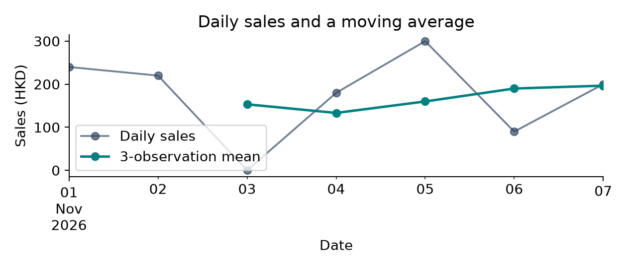
A rolling mean smooths short-term variation. Change the window from 3 to 2 or 4, then compare the curve and the number of initial missing values.
Create the dates first:pd.date_range(start="2026-11-01", periods=7, freq="D") creates a DatetimeIndex containing seven consecutive calendar dates, November 1 through November 7.
Argument
Meaning in this example
start="2026-11-01"
The first date is November 1, 2026.
periods=7
Create seven dates, including the first date.
freq="D"
Move forward one calendar day each time; D means daily.
Save these dates as dates. Using index=dates pairs each sales value with its date. This function creates dates; it does not create sales values or fill missing sales.
Rolling Sums and Standard Deviations
A rolling sum measures recent total sales. A rolling standard deviation describes recent variation. Both need a defined window and units.
Incomplete Windows and min_periods
min_periods=1 allows an early mean using the available values. That first output is a one-observation mean, even though the maximum window size is 3.
Three Observations versus Three Calendar Days
On irregular dates, .rolling(3) and .rolling("3D") use different windows. The default right-closed time window excludes an observation exactly at its left boundary.
Cumulative Sales: Keep Adding from the Start
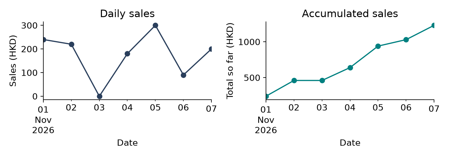
.cumsum() retains all observations from the beginning through the current row. It answers “How much so far?” rather than “How much in the recent window?”
Chart: Daily and Accumulated Sales
Compare sales on each day with sales accumulated so far using two separate charts. Use the familiar Series methods .plot.bar() and .plot(), with plt.title(), plt.xlabel(), and plt.ylabel() to label each chart.
Cumulative Maximum and Minimum
Cumulative means using every observation from the first row through the current row.
.cummax() gives the cumulative maximum: the highest value observed so far.
.cummin() gives the cumulative minimum: the lowest value observed so far.
A cumulative maximum can stay unchanged when the current sales value falls; a cumulative minimum can stay unchanged when the current sales value rises.
.cumprod() means cumulative product: multiply all values from the first row through the current row. It returns one product for each row.
For [2, 3, 4], the cumulative products are [2, 2 × 3, 2 × 3 × 4] = [2, 6, 24].
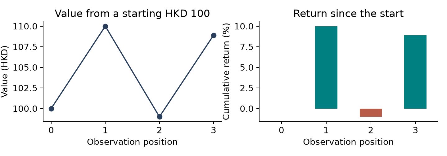
For returns, first calculate each growth factor as 1 + return. Then use .cumprod() to multiply the factors. Subtract 1 from the product to obtain the cumulative return.
Row
Return
Growth factor
Cumulative product
Cumulative return
0
+10%
1.10
1.10
1.10 − 1 = +10%
1
−10%
0.90
1.10 × 0.90 = 0.99
0.99 − 1 = −1%
2
+10%
1.10
1.10 × 0.90 × 1.10 = 1.089
1.089 − 1 = +8.9%
Multiply the growth factors; do not add the returns.
From Prices to Cumulative Returns
The first price has no return from a previous observation. Set the known starting value to 100 for this complete-price example, then compound subsequent growth factors.
Financial Example: S&P 500 Data
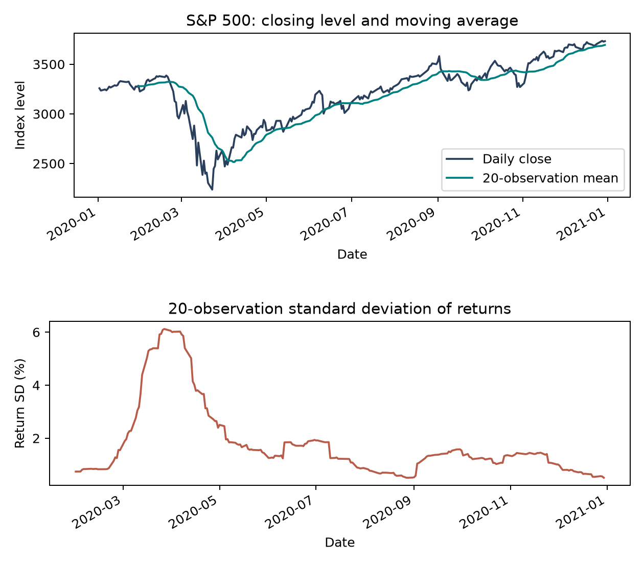
Load the course’s 2020 S&P 500 snapshot. Select dates, calculate fractional returns, and compare a price moving average with a returns standard deviation.
Financial Chart: Prices and Return Variation
Read two separate charts made with the familiar .plot() method:
Closing level and moving average: the blue line shows the S&P 500 closing level on each date. The teal line shows the mean of the most recent 20 observations. The vertical axis measures index level.
Variation in daily returns: the red line shows the standard deviation of the most recent 20 returns. Multiplying by 100 displays it as a percentage. A higher value means the recent daily percentage changes varied more.
Change window = 20 to window = 10, then run again and compare both charts.
Extension: A Running Peak and Drawdown
Drawdown compares the current price with its highest value so far: price / running peak − 1. It is zero at a peak and negative below that peak.
Rolling and Cumulative Answer Different Questions
Compare the last three observations with all observations so far. Select a rolling sum for recent sales; select a cumulative sum for progress since the beginning.
In-Class Practice: Recent Sales and Total Sales
Compute the three-observation rolling mean and cumulative sales. Print the final values and explain why they answer different questions.
Expected final rolling mean: 400 HKD per observation. Expected cumulative total: 1500 HKD.